Roughness and microslicing

Interfacial roughness

The slab model that has been discussed has a clear problem, it that it implies perfectly flat interfaces between different materials. These cannot exist in real materials, therefore it is necessary to enable some roughness between the interfaces in our model. There are a range of functions that can be used to implement interfacial roughness in slab modelling. However, the most common is the use of an error function [NevotC80].

We can visualise a typical error function roughness below, where we show the silicon dioxide on silicon sample from before with a roughness of \(0\) Å between each layer and with a roughness of \(10\) Å between each layer.

Note

The code used to obtain the scattering length density profile with roughness can be found in the helper.py module.

import numpy as np
import matplotlib.pyplot as plt
from matplotlib.patches import Rectangle
from helper import sld_with_roughness, microslicing, abeles, abeles_with_roughness

beta = np.array([0 + 0j, 4.186e-6 + 0j, 2.871e-6 + 0j])
d = np.array([0, 200, 0])
sigma = np.array([0, 0])
sigma2 = np.array([10, 10])
plt.plot(*sld_with_roughness(beta, d, sigma), label='0 Å')
plt.plot(*sld_with_roughness(beta, d, sigma2), label='10 Å')
plt.xlabel('$z$ (Å)')
plt.ylabel(r'$\beta(z)$ (Å$^{-2}$)')
plt.legend()
plt.show()

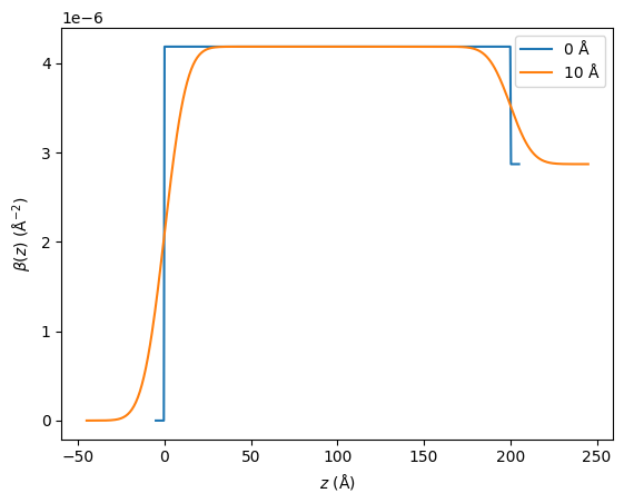
We can see that this roughness creates some smoothing of the interface between the layers. We must modify the Abelès matrix formalism discussed previously to account for this smoothing. This is achieved by adapting the calculation of the Fresnel reflectance,

(20)\[r_{n, n+1}(q) = \frac{k_n(q) - k_{n+1}(q)}{k_n(q) + k_{n+1}(q)} \exp{(-2k_nk_{n+1}\sigma_{n,n+1}^2)},\]

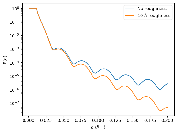
where, \(\sigma_{n, n+1}^2\) is the roughness width between the interfaces. We can observe the effect that this interfacial roughness has on the resulting reflectometry profile, shown below.

Note

Again, the code used to find the reflectivity with roughness (and without) can be found in the helper.py module.

q = np.linspace(0.001, 0.2, 500)
beta = np.array([0 + 0j, 4.186e-6 + 0j, 2.871e-6 + 0j])
d = np.array([0, 200, 0])
r = abeles(q, beta, d)
sigma = np.array([10, 10])
r_with_roughness = abeles_with_roughness(q, beta, d, sigma)

plt.plot(q, r, label='No roughness')
plt.plot(q, r_with_roughness, label='10 Å roughness')
plt.xlabel('q (Å$^{-1}$)')
plt.ylabel('R(q)')
plt.yscale('log')
plt.legend()
plt.show()

Problems with interfacial roughness

This method for considering interfacial roughness between two layers is not perfect, and if used incorrectly can introduce unphysical artefacts to our reflectometry calculation. Consider the example shown below, where there is a \(10\) Å layer of nickel on a substrate of silicon. The roughness between the nickel and air is increased from \(3\) Å to \(7\) Å with no roughness between the nickel and silicon.

beta = np.array([0 + 0j, 9.4245e-06 + 0j, 2.074e-6 + 0j])
d = np.array([0, 10, 0])
sigma3 = np.array([3, 0])
sigma5 = np.array([5, 0])
sigma7 = np.array([7, 0])

fig, ax = plt.subplots(1, 2, figsize=(12.8, 4.8))

ax[0].plot(*sld_with_roughness(beta, d, sigma3), label='3 Å')
ax[0].plot(*sld_with_roughness(beta, d, sigma5), label='5 Å')
ax[0].plot(*sld_with_roughness(beta, d, sigma7), label='7 Å')
ax[0].set_xlabel('$z$ (Å)')
ax[0].set_ylabel(r'$\beta(z)$ (Å$^{-2}$)')
ax[0].legend()
ax[0].add_patch(Rectangle((8.5, 1.25e-6), 6, 1e-6, edgecolor='r', fill=False))

ax[1].plot(*sld_with_roughness(beta, d, sigma3), label='3 Å')
ax[1].plot(*sld_with_roughness(beta, d, sigma5), label='5 Å')
ax[1].plot(*sld_with_roughness(beta, d, sigma7), label='7 Å')
ax[1].set_xlabel('$z$ (Å)')
ax[1].set_ylabel(r'$\beta(z)$ (Å$^{-2}$)')
ax[1].set_xlim(8.5, 14.5)
ax[1].set_ylim(1.25e-6, 2.25e-6)
ax[1].legend()

plt.show()

Note

A common rule of thumb for using Nevot-Croce is that the roughness on an interface should be no more than \(20\) % of the thickness of the shortest slab.

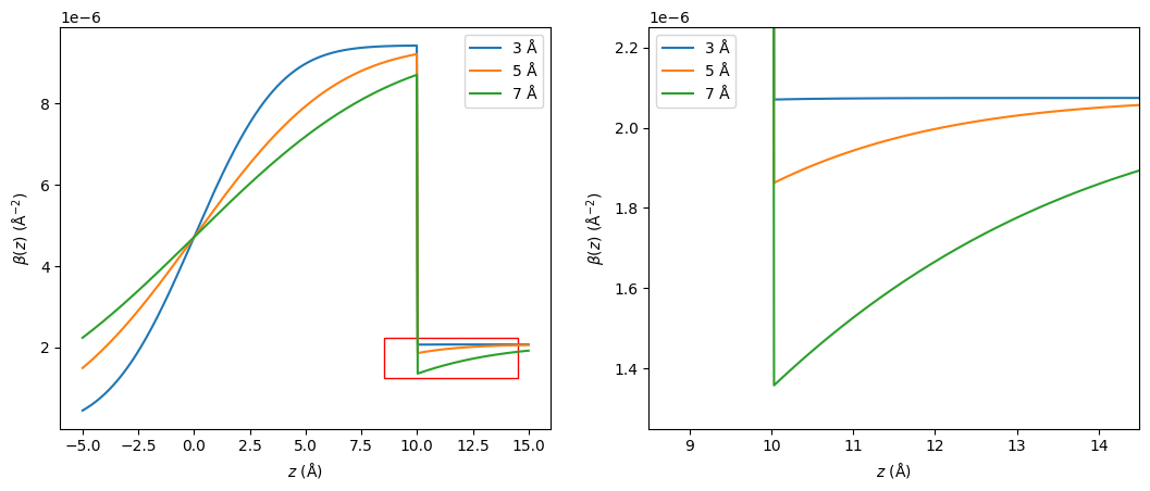
The red rectangle in the left-hand plot identifies the region that is shown in the right-hand plot. From these figures, it is clear that the roughness between the nickel and air is leaking through to the nickel-silicon interface. This can lead to an unphysical interpretation of our system if we interrogate the scattering length density profile. Additionally, given that the roughness parameter only influences the Fresnel reflectance between two interfaces, this “leaking” through it not reflected in the resulting calculated data.

Microslicing

It is still possible that we would like to be able to simulate such a scattering length density profile as is shown above, accurately. Therefore, there must be a methodology to work around this problem with the Nevot-Croce approach. This method is microslicing, where the scattering length density profile is described as a series of very thin layers with no roughness between them. Consider the plot shown below, which presents the same interface as before, however, this time comparing the Nevot-Croce approach and microslicing.

Note

The microslicing code can be found in the helper.py module.

beta = np.array([0 + 0j, 9.4245e-06 + 0j, 2.074e-6 + 0j])
d = np.array([0, 10, 0])
sigma7 = np.array([7, 0])

fig, ax = plt.subplots(1, 2, figsize=(12.8, 4.8))

ax[0].plot(*sld_with_roughness(beta, d, sigma7), label='Nevot-Croce')
ax[0].step(*microslicing(beta, d, sigma7, 0.5), label='Microslicing')
ax[0].set_xlabel('$z$ (Å)')
ax[0].set_ylabel(r'$\beta(z)$ (Å$^{-2}$)')
ax[0].legend()
ax[0].add_patch(Rectangle((8.5, 1.25e-6), 6, 1e-6, edgecolor='r', fill=False))
ax[0].set_xlim(-7.5, 17.5)

ax[1].plot(*sld_with_roughness(beta, d, sigma7), label='Nevot-Croce')
ax[1].step(*microslicing(beta, d, sigma7, 0.5), label='Microslicing')
ax[1].set_xlabel('$z$ (Å)')
ax[1].set_ylabel(r'$\beta(z)$ (Å$^{-2}$)')
ax[1].set_xlim(8.5, 14.5)
ax[1].set_ylim(1.25e-6, 2.25e-6)
ax[1].legend()

plt.show()

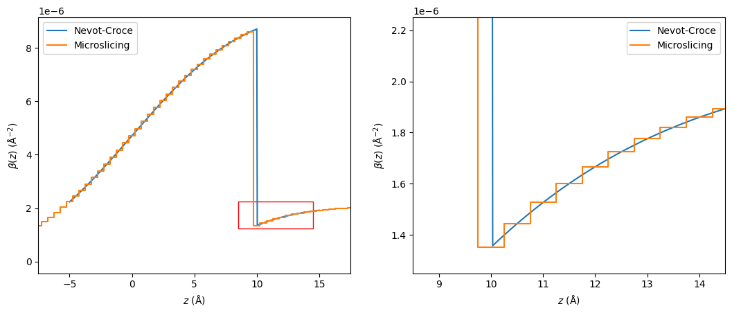
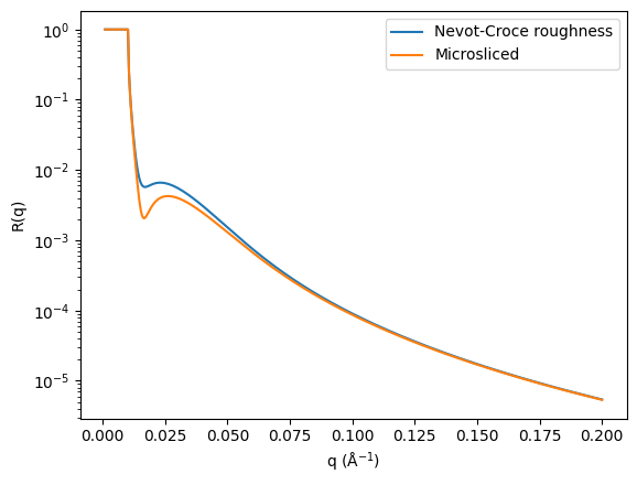
Notice that now the system is a series of layers with a thickness of \(0.5\) Å each. This means that by applying the Abelès matrix formalism to this profile and ignoring any roughness, the reflectivity will be that for the (admittedly unphysical) system where the roughness does leak through. Below, we compare two reflectometry profiles using the error function roughness and where the microsliced scattering length density profile is used. To show clearly the impact of the Nevot-Croce approach being inaccurate, we show data where the roughness has a width of \(50\) Å.

q = np.linspace(0.001, 0.2, 500)
beta = np.array([0 + 0j, 9.4245e-06 + 0j, 2.074e-6 + 0j])
d = np.array([0, 10, 0])
sigma7 = np.array([50, 0])
r_nevot_croce = abeles_with_roughness(q, beta, d, sigma7)
d_microsliced, beta_microsliced = microslicing(beta, d, sigma7, 0.5)
r_microsliced = abeles(q, beta_microsliced + 0j, np.ones_like(beta_microsliced) * 0.5)

plt.plot(q, r_nevot_croce, label='Nevot-Croce roughness')
plt.plot(q, r_microsliced, label='Microsliced')
plt.xlabel('q (Å$^{-1}$)')
plt.ylabel('R(q)')
plt.yscale('log')
plt.legend()
plt.show()