How do we maximise the likelihood?#
Now that there is a metric we will use to assess the quality of agreement between our model and our data, we can consider how we find the maximum likelihood for a given system. In this section, we will look at a couple of common methods for likelihood maximisation that are used in neutron reflectometry analysis. These methods take on two flavours, that we will investigate in turn.
Gradient methods#
The first method for likelihood maximisation that one will encounter in reflectometry analysis are gradient methods. These are optimisation algorithms that aim to maximise the likelihood by starting from the initial guess position and finding the local gradient. Once this is determined, the gradient method looks to move the current guess uphill to eventually reach some nearby maximum value. We can see a simple example of this below, where we find the maximum likelihood by a gradient method for a two-dimensional normal distribution. A range of gradient methods exist, but in general, they all try to find the maximum be considering local gradients.
import numpy as np
import matplotlib.pyplot as plt
from scipy.stats import multivariate_normal
from scipy.optimize import minimize
mv = multivariate_normal([3.000, 1.000], [[0.033 , -0.167], [-0.167,  1.092]])
gradient_v = []
def gradient_callback(current_theta: np.ndarray) -> None:
    gradient_v.append(current_theta)

def nll(theta: np.ndarray) -> float:
    return -mv.logpdf(theta)

res = minimize(nll, [2.6, 3], callback=gradient_callback, method='Nelder-Mead')
gradient_v = np.array(gradient_v)
x = np.linspace(2.6, 3.4, 1000)
y = np.linspace(-1.5, 3.5, 1000)
X, Y = np.meshgrid(x, y)
plt.contourf(X, Y, mv.pdf(np.array([X, Y]).T).T)
plt.plot(gradient_v[:, 0], gradient_v[:, 1], 'k-')
plt.xlabel('$m$')
plt.ylabel('$c$')
plt.colorbar(label='$\ln\mathcal{L}$')
plt.show()
print('Maximum:', res.x)
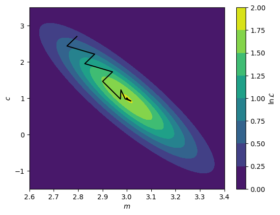
Maximum: [2.99999727 0.99998503]
We can see above that the black line, indicating the path of the solution towards the maximum, moves in a rational path up towards the maximum, following the regions of an increasing gradient. Eventually, after a number of steps, the maximum is found.
Gradient methods are effective for the discovery of local maxima, however, for more complex model-dependent analysis, this can be a problem. If the maximum that is found by the gradient method is not the global maxima, then it is not possible for these algorithms to easily go back “downhill”. This means that the starting position of the algorithm is very important.
Consider the two routes shown below on the multi-modal (more than one maximum) likelihood function. The blue line starts near to the local maximum at \((3, 0)\) and therefore the gradient approach is used, it is this maximum that is found. However, when the algorithm is started from \((10, 5)\) (orange line), the true global maximum at \((8, 2)\) is found instead. It is clear that for the non-unique analyses of neutron reflectometry, we desire a global optimisation approach.
mv1 = multivariate_normal([3, 0], [[4, 2], [-2, 4]])
mv2 = multivariate_normal([8, 2], [[2, 1], [1, 2]])

def nll(theta: np.ndarray) -> float:
    return -(mv1.pdf(theta) + mv2.pdf(theta))

x = np.linspace(0, 11, 1000)
y = np.linspace(-4, 5, 1000)
X, Y = np.meshgrid(x, y)
plt.contourf(X, Y, mv1.pdf(np.array([X, Y]).T).T + mv2.pdf(np.array([X, Y]).T).T)
gradient_v = []
res1 = minimize(nll, [1, 3], callback=gradient_callback, method='Nelder-Mead')
gradient_v = np.array(gradient_v)
plt.plot(gradient_v[:, 0], gradient_v[:, 1], '-')
gradient_v = []
res2 = minimize(nll, [10, 5], callback=gradient_callback, method='Nelder-Mead')
gradient_v = np.array(gradient_v)
plt.plot(gradient_v[:, 0], gradient_v[:, 1], '-')
plt.xlabel('$x$')
plt.ylabel('$y$')
plt.colorbar(label='$\ln\mathcal{L}$')
plt.show()
print('Blue Maximum:', res1.x)
print('Orange Maximum:', res2.x)
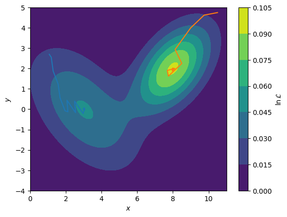
Blue Maximum: [ 3.04493869 -0.02614057]
Orange Maximum: [7.9957561  1.99615666]
Stochastic methods#
The most common form of global optimisation methods are the stochastic methods, where stochastic means random. There are a variety of these methods, such as particle swarm, which moves in the semi-random fashion analogous to a swarm of insects, or evolutionary algorithms, which are inspired by biological evolution in order to find the optimum. The most commonly applied in neutron reflectometry model optimisation is the differential evolution method [Bjorck11, SP97, WPMB99].
In the figure below, we show the application of a differential evolution algorithm with a population of \(8\) (however, the optimisation route of the \(4\) best members are shown). It is clear that the methodology results in a more complete interrogation of the complex optimisation space. Typically once a solution is found using the differential evolution, this is further optimised with a gradient descent method to find the maximum global likelihood. This is necessary as, as we can see from the overall maximum, the differential evolution will not find the absolute maximum alone.
from helper import differential_evolution

x = np.linspace(0, 11, 1000)
y = np.linspace(-4, 5, 1000)
X, Y = np.meshgrid(x, y)
plt.contourf(X, Y, mv1.pdf(np.array([X, Y]).T).T + mv2.pdf(np.array([X, Y]).T).T)
res = differential_evolution(nll, ((0, 11), (-4, 5)))
top4 = np.argsort(nll(res[-1].T))[:4]
plt.plot(res[:, 0, top4], res[:, 1, top4], '-')
plt.xlabel('$m$')
plt.ylabel('$c$')
plt.colorbar(label='$\ln\mathcal{L}$')
plt.show()
print('Overall Maximum:', res[-1].T[np.argmax(nll(res[-1].T))])
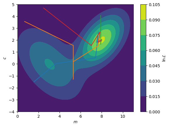
Overall Maximum: [7.9106823 1.9518762]
It is important to note that as the dimensionality to a fitting problem increases, as the number of free parameters in our model increases, it will become harder and harder to find an optimised solution. Therefore, we should carefully consider which parameters in a model are allowed to vary in the fitting process, ensuring that the minimum number of parameters are changing. There are some important considerations that feed into this, for example, that having more isotopic contrasts of neutron reflectometry data means that more parameters can be varied.
Once some maximum likelihood is found, it is possible to probe the shape of that maximum and draw conclusions about the robustivity of the result. Additionally, the maximum number of free parameters that a given dataset(s) can describe is quantifiable, however, very computationally intensive [TKH+19].